The average work done due to friction in the gear mesh can then be described as the average work done in one mesh cycle of the gear.
 (4)
(4)
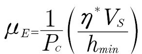
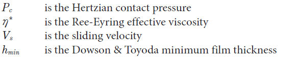
where
Validation of the model was done using measured gear mechanical power loss data taken from various surface roughness pinion-gear pairings including equivalent surface pairings (surfaces machined the same) and dissimilar surface pairings (surfaces finished differently). Predictions matched the measured mechanical power loss closely for all pairings and conditions. Figure 1 shows the results of this comparison as adapted from (Ref. 1).
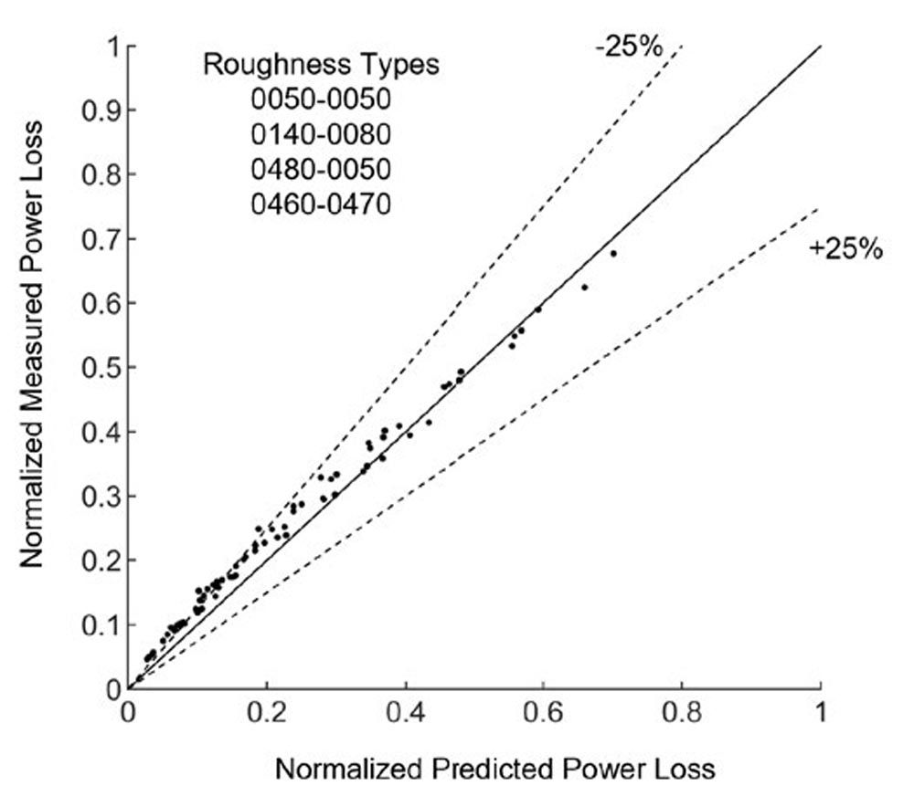
Figure 1—Model predicted power loss as compared to measured mechanical power loss. Adapted from Ref. 1.
Simulation Matrix and Roughness Profile Analysis
The gear mechanical power loss model is used to help understand how average gear mechanical power loss is affected by both pairings of like surfaces (ex: ground pinion and gear flanks from the same grinder) but also pairs of unlike roughnesses (e.g., ground pinion mated with a polished gear). Gears finished from various processes were measured off a Talysurf I-20 profilometer to extract the 2D roughness profile. Measurements and filters were made to conform to ISO 4288:1996 (Ref. 8). Six different traces covering a span of Ra=0.036 nm to Ra=0.450 nm. These profiles are listed in Table 1.
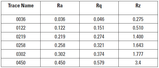
Figure 2 shows a visual comparison of the magnified roughness profiles. The scale is consistent between all measurements. A 1.5 mm segment has been extracted from the full measurement for display purposes. Full measurements were used in all calculations.
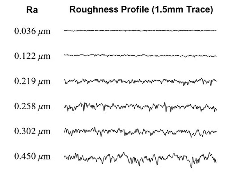
Figure 2—Magnified roughness profiles.
It is important to note that McCool’s parameterization of the measured roughness amplitudes assumes the roughness amplitudes are Gaussian in nature and that the asperity tip radii are equal for all asperities and density is constant. This at minimum precludes the model from comprehending the effects of local surface defects on gear mechanical power loss such as from scratches or from irregular machining patterns. The surfaces used for validation of the model all had roughness amplitudes that conformed reasonably well to a Gaussian distribution with some exceptions at the extreme valleys and peaks of the material. Goodness-of-fit can be checked visually by plotting the surface heights on a Normal Probability Plot. If the data conforms to the normal distribution, then it shall follow a straight line. Deviations from the normal distribution are shown as deviations from a straight line. Normal Probability Plots are shown in Figure 3 for each of the six roughness profiles.
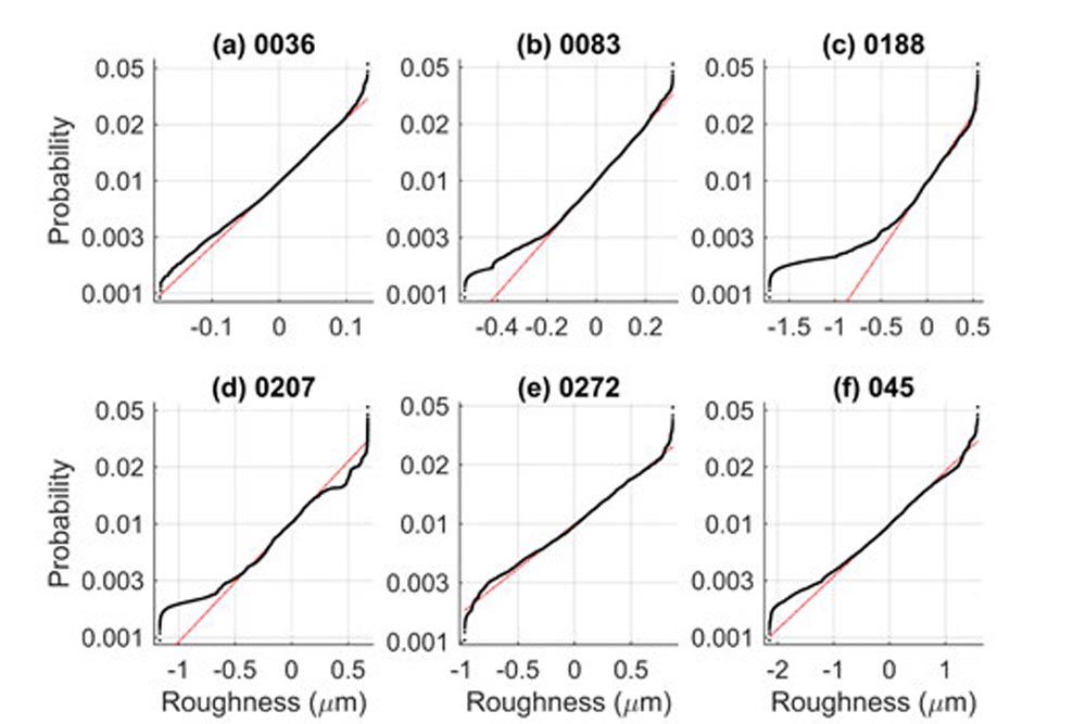
Figure 3—Normal probability plots for the roughness profiles.
The bulk of the material for all traces conforms closely to a Gaussian distribution. For all profiles, material at the extreme valleys and peaks exhibits several outliers consistent with roughness profiles used in the model validation of Ref. 1. The roughness profiles do not exhibit any significant deviation from the normal distribution in between the extreme peaks and valleys which would indicate surface defects or non-repetitive surface asperity characteristics.
A full factorial of simulations is performed using the previously described mechanical power loss model and the six shown surfaces. This results in 21 unique parings of surfaces and simulations according to Table 2.
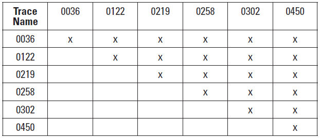
Table 2—Surface pairing for simulation runs.
Simulations were done using gear specifications according to Table 3.
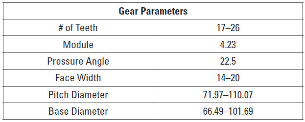
Table 3—Gear parameters used for power loss simulations.
Simulated operating conditions are typical of automotive applications. Oil viscosity parameters belong to a typical automotive transmission fluid. For each of the 21 surface paring combinations, a full factorial of three torques (50, 100 and 150 Nm) and six speeds (500, 1000, 1500, 2000, 2500 and 3000 rpm) as shown in Table 4 were used for a total of 18 predictions per surface pairing combination. In total, 378 different conditions were simulated as part of this study. The computing time required to run these simulations was less than 1 minute.
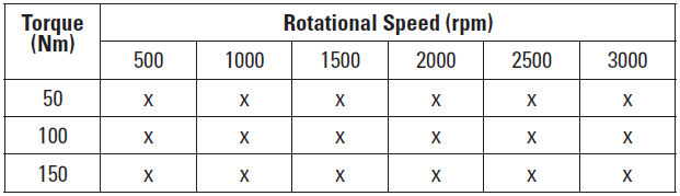
Table 4—Simulation operating conditions.
Effect of Various Surface Roughness Parings
The results of the modeling are shown for equivalent surface pairings (0036-0036, 0122-0122, 0219-0219, 0258-0258, 0302-0302, 0450-0450) in Figure 4. Power loss magnitudes have been normalized such that the focus of this study is correlation and trend rather than magnitudes of the arbitrary gear design simulated. The general correlation of power loss to operating torque and speed is the same in all pairings. Peak power loss occurs at the highest speed and torque condition for all pairings. As the roughness increases power loss is seen to increase.
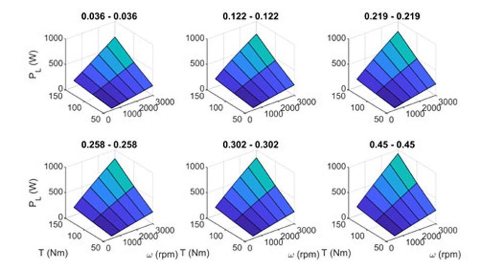
Figure 4—Predicted mechanical power loss for equivalent surface parings.
Similarly, mechanical power loss predictions for all surfaces paired with the smoothed surface (0036) are shown in Figure 5. This compares the correlation of mechanical power loss to torque and speed against similar surface parings and dissimilar surface pairings. Again, power loss correlates in a similar manor as torque and speed are changed.
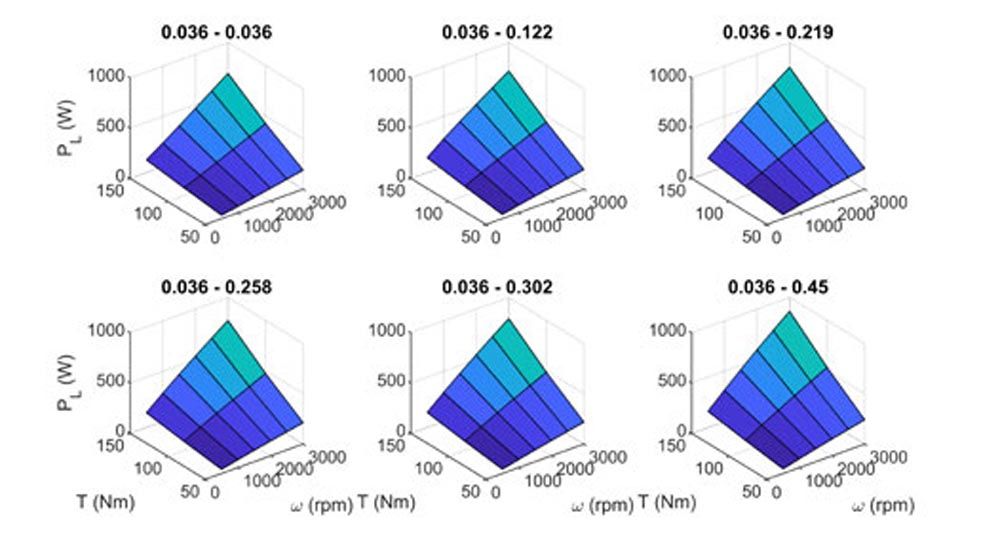
Figure 5—Predicted mechanical power loss for 0036 surface parings.
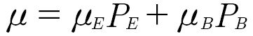
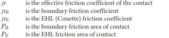
The primary variable of interest from the model predictions, besides mechanical power loss itself is the prediction of the area asperity contact ratio. This alone weights the effective friction coefficient between boundary friction μB=0.1 and EHL friction (approximated as Couette Flow) and describes the relative contributions of each to the effective friction coefficient. Extreme operating conditions in terms of fluid film thickness will be at high torque, low speed for low film thickness and high speed, low torque for high film thickness. This is observed in the boundary area contact ratio for both equivalent surface pairings and dissimilar surface pairings from the model as shown in Figure 6 and Figure 7, respectively.
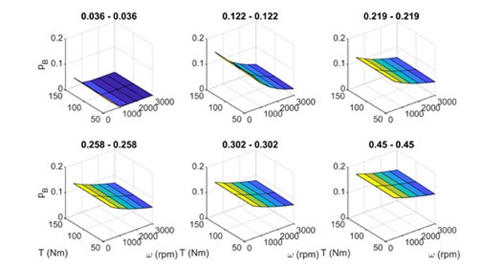
Figure 6—Boundary area contact ratio for equivalent surface pairings.
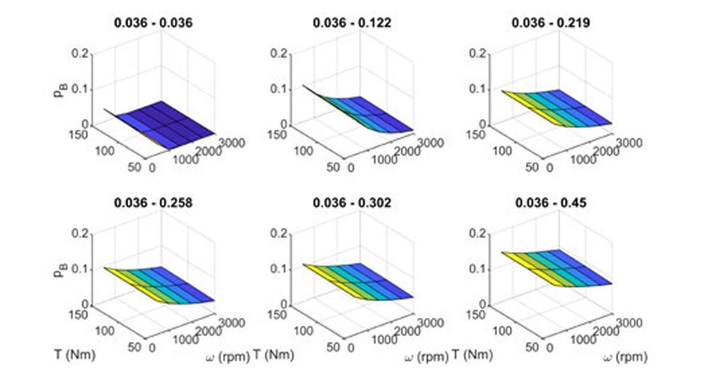
Figure 7—Boundary area contact ratio for 0036 surface pairings.
For surface parings in which a smoother surface is paired with a rough surface, the boundary area contact ratio is lower as compared to paring two of the rough surfaces as expected. It is also noted that within the operating conditions explored in this study only the smoothest surface pairing of 0036-0036 exhibits no boundary asperity contact at the higher speeds although it is expected that the 0036-0122 pairing would display this property if operating speeds were extended.
Composite roughness is an often-cited metric of roughness conditions in EHL contact, particularly when used as part of the film parameter m. Composite roughness is defined as
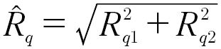 (5)
(5)
Composite Roughness metrics for the 21 surface pairings are shown in Table 5.
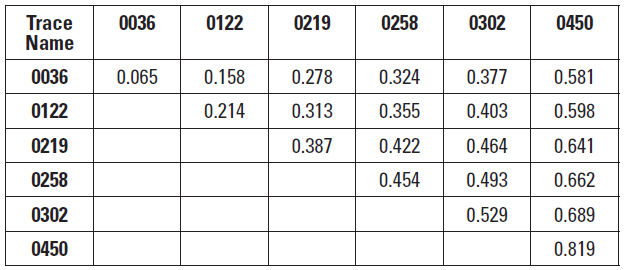
Table 5—Composite roughness ( ).
).
The film parameter λ is defined as
 (5)
(5)
where
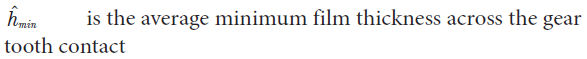
Normalized power loss vs composite roughness is shown for each of the 378 simulation conditions in Figure 8 at (a) 50 Nm, (b) 100 Nm and (c) 150 Nm 17T pinion torque. At any given operating condition (torque and speed) there is an approximate linear relationship between the composite roughness and mechanical power loss within the range of operating conditions used here. From a design standpoint this means that if operating conditions on the transmission are fixed, the transmission designer may approximate changes to mechanical loss if the mechanical loss at two different composite roughness values are known. This helps to avoid unnecessary costs in efficiency testing. However, composite roughness does not provide any information on how mechanical power loss will vary with torque and speed.
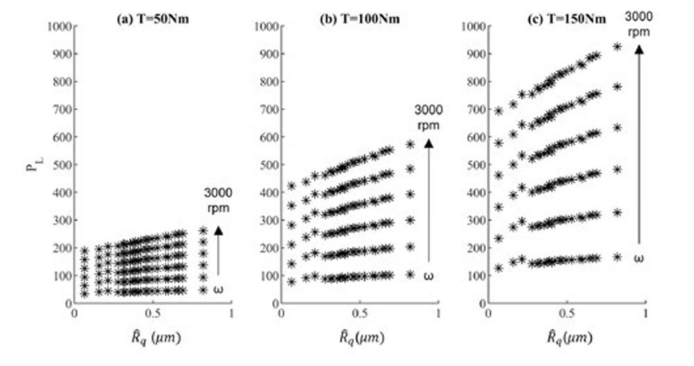
Figure 8—Predicted power loss vs. composite roughness.
Predicted mechanical power loss is plotted against the film parameter λ in Figure 9. Mechanical power loss shows similar bands corresponding to the simulated torque and speed conditions. At any given torque and speed condition the Dowson and Toyoda predicted average minimum film thickness is equal for all roughness pairings as it is assumed independent of roughness. This means that at any given operating condition λ is solely a function of the composite roughness and increases as composite roughness decreases. At any given operating condition in which film thickness is high enough to present film parameters of >1, predicted mechanical power loss shows a very little decrease with a further increase of the film parameter. This indicates there is little gain from an efficiency standpoint from further smoothening of the surfaces once the film parameter is equal to or greater than one for the operating conditions used in this study. There is, however, a speed dependence on the precise λ corresponding to equivalent slopes in the power loss vs film parameter plots. Higher operating speeds will result in higher film parameter values for equal diminishing returns in efficiency gains.
Figure 9—Predicted power loss vs. film parameter.
The same deficiency exists with the film parameter as with the composite roughness for the prediction of mechanical power loss. This is because the film parameter itself still provides no correlation to the magnitude of power loss with changes in torque and speed and only correlates to roughness conditions at a single operating condition. This is even though the film parameter accounts for the changes in film thickness due to operating conditions.
The observed boundary area contact ratios for the operating conditions and roughness amplitudes were well away from both 0 (no asperity contact) and 1 (purely asperity contact) indicating the gear teeth would be operating in mixed lubrication conditions. When considering the linear trend discussed in Figure 8 of power loss vs composite roughness it must be annotated that this is true only in the mixed lubrication condition. If roughness were to continue to increase well past 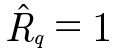 , the film parameter would approach zero (λ →0), and eventually, the boundary area contact ratio would approach 1 (PB→1) indicating almost pure asperity contact. At this point, the effective friction coefficient is almost purely dependent on the boundary friction coefficient. Furthermore, increasing the roughness amplitudes even more would not affect that friction coefficient in a way comprehendible by this model approach. This means that at some large composite roughness value, the trend of a linear increase in power loss with composite roughness would break, and predicted power loss would be equivalent even as composite roughness is increased.
Similarly, as roughness is dropped the film parameter will approach infinity (λ →∞), and the boundary area contact ratio will go to zero (PB→0) indicating that the effective friction coefficient will be purely dominated by fluid shear (within the assumptions of this model). This friction coefficient will also be constant for each operating condition and further reductions in roughness will not result in significant changes to mechanical power loss. Again, the linear trend of power loss with composite roughness will break at very low roughness values and the predicted power loss would be equivalent even as composite roughness is decreased.
This discussion suggests that mechanical power loss will have a purely linear relationship with the boundary area contact ratio. This is shown in Figure 10 and that trend is observed. It is again seen that most of the contacts operate in a mixed lubrication condition with few conditions having no asperity contact. This condition with no asperity contact is the 0036-0036 condition at 1500 rpm and above for all torque levels.
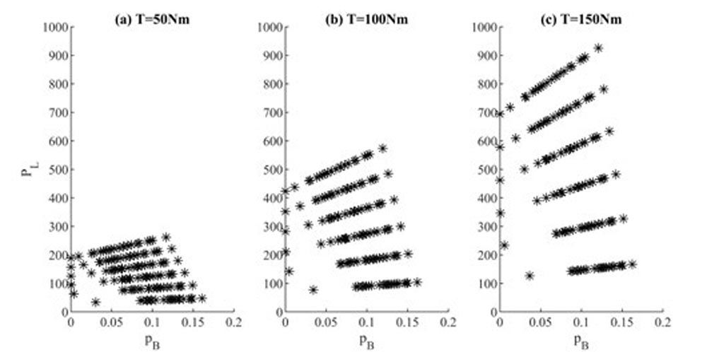
Figure 10—Predicted power loss vs. boundary area contact ratio.
Summary and Conclusions
A model developed by Ref. 1 for the prediction of gear mechanical power loss was used to investigate 378 unique gear operating conditions consisting of 21 different pairings of gear surface roughness. Applied torque varied from 50 to 150 Nm and operating speed varied from 500 to 3000 rpm. Surface roughness profiles varied from Ra=0.036 μm (Rq=0.046 μm) to Ra=0.450 μm (Rq=0.579 μm). All roughness profile amplitudes were shown to conform to a Gaussian distribution for the bulk of the material surface heights consistent with the requirements for the power loss model.
Power loss was shown to increase almost linearly with composite roughness at any given torque and speed operating condition. However composite roughness alone does not describe the relationship between power loss to torque and speed. This does allow for reduced experimental need with respect to high-resolution increments in surface roughness amplitude and shifts the focus to experimental testing of a wide range of operating torque and speeds.
With respect to the film parameter, it is observed that past m=1 at any given operating condition, and very little reduction in mechanical power loss takes place. This in turn means that further smoothening of the surfaces will not result in a substantial gain in mechanical efficiency. However, the correlation between power loss and operating conditions cannot be determined from the film parameter, and experimentation or modeling is required.
Simple metrics such as the composite roughness or film parameter can be useful when determining relative mechanical power loss at a fixed operating condition. However, they require experimentation or modeling to understand the effect of operating conditions. The model presented performs well with roughness profiles conforming to a normal distribution, but caution is urged when presented with problems arising from the presence of surface defects or irregularities. Under regular circumstances, the model can provide results for thousands of operating conditions and roughness profile pairing with minimal computational overhead making it useful for early design phase decision-making.

References
- Hong, I., Aneshansley, E., Chaudhury, K., and Talbot, D., “Stochastic Microcontact Model for the Prediction of Gear Mechanical Power Loss,” Tribol. Trans.
- 2016, Windows-LDP, Load Distribution Program, The Gear and Power Transmission Research Laboratory, The Ohio State University, Columbus, Ohio.
- Dowson, D., and Toyoda, S., 1978, “A Central Film Thickness Formula for Elastohydrodynamic Line Contacts,” Proceedings of the 5th Leeds-Lyon Symposium, London, pp. 60–65.
- Greenwood, J. A., and Williamson, J. B. P., 1966, “Contact of Nominally Flat Surfaces,” Proc. R. Soc. London. Ser. A. Math. Phys. Sci., Vol. 295, No. 1442, pp. 300–319.
- McCool, J. I., 1987, “Relating Profile Instrument Measurements to the Functional Performance of Rough Surfaces,” J. Tribol., Vol. 109, No. 2, pp. 264–270.
- Tallian, T., 1972, “The Theory of Partial Elastohydrodynamic Contacts,” Wear, 21, pp. 49–101.
- Wu, S., and Cheng, H. S., 1991, “A Friction Model of Partial-EHL Contacts and Its Application to Power Loss in Spur Gears,” Tribol. Trans., Vol. 34, No. 3, pp. 398–407.
- ISO, 1996, ISO 4288:1996—Geometrical Product Specifications (GPS)—Surface Texture: Profile Method—Rules and Procedures for the Assessment of Surface Texture.


 (1)
(1)
 (2)
(2)
 (3)
(3)