Cross-Correlation of Design Variables for Epicyclic Systems

The automotive industry pays great attention to the concept of power density and friction losses concerning mechanical transmission systems. Moreover, installation benefits and weight reduction are achieving higher density power. Another important study is about mechanical efficiency: their reduction allows to minimize the heat exchange; the power dissipation problem—produced by friction—must be addressed. Therefore, the gear designer is obligated to incorporate additional cooling systems, or with higher capacity, to address this problem.

Nowadays, electrical units must operate at higher speeds, and they also must manage two-way loading operations, especially hybrid transmissions. The combination of speed and torque must be managed by designers, considering load histories, and evaluating them appropriately.

In this context, the planetary gear systems meet the requirements of compactness and allow obtaining a high power density, especially compared with classic transmission systems obtained by cylindrical gear pairs. High transmission ratios can be reached thanks to these systems; as the target transmission ratio increases the comparison of mechanical epicyclic systems shows even more complex advantages. It is the task of the gear designer to choose the most suitable solution for his application. 

Today lacks (focusing on the design of epicyclic gear drive systems) a tool that allows evaluating a series of them with defined constraints. The layout of interest chosen for this analysis involves a fixed ring gear, sun gear in speed out, and carrier as input. The study presented in this paper aims to show a flow of operation that allows the systematic study of gear train families, and it’s able to balance the pros and cons through correct visualizations.

Variable objectives and constraints will be defined, as in any optimization process (Ref. 1). The generated variants will then be analyzed with different criteria. The article focuses on the methods of generation of variants and the graphical mode of evaluation of results (matrix plot) (Ref. 2).

Background

First, it is necessary to develop a tool that allows generating multiple design solutions for macro settings of different planetary gears. To make the creation of different solutions, as general as possible, interest variables are imposed in acceptability ranges, with defined constraints. The macro settings information, that the user can decide includes the variability range of the number of teeth of ring and planet, module, numbers of planets, and minimum acceptable number of teeth on the sun. Based on these settings, design solutions are generated—and will be evaluated for the exact definition of the teeth. The study presented shows variables that have been chosen not to change, but by increasing that—and possible combinations accordingly—it is possible to introduce additional ranges to find more sensitivities beyond those chosen.

It should be noted that for the same epicyclic system, two solutions are tested by choice, with planet number of teeth z and z−1. Through the shift profile modification, it is always possible to guarantee both design solutions, achieving different resistance and performance targets—which will be evaluated later.

At this stage, the attention is also directed to the possible behavior of the dynamic system. It is well known the different dynamic behavior of the epicyclic system between sequential or symmetric gear mesh. For a deeper understanding of this, please refer to the specialized text (Ref. 3); summarizing the theme, with different planets meshing with the sun, sun forces arise from the superposition of effects of each gear meshing contact. The mesh sequence, i.e., the phasing between the individual meshes, is an important parameter. The forcing phase allows the defining of two different assembly-forcing conditions, symmetric or sequential mesh sequences. In practice the different layout setting allows to have forcing mostly rotational or translational; the in-depth study of the modal analysis allows the designer to offer a more important overview of the whole system, to detect which are the most dangerous eigenmodes, if rotational or translational modes (Ref. 4). 

From general practice, the symmetric solution is preferred, but in reality, it is the dynamic study that defines which solution is the best. 

For what concerns this paper today, the mathematical condition that allows to have one solution instead of another is evaluated: it will be a variable associated with each proposal.

One of the most important design engineering choices (Ref. 5) references the basic rack tooth profile, to which the various coefficients of addendum, dedendum, and root radius are linked. In any case, the designer can decide to modify these parameters as preferred. In the current study the standard ISO 53, Type A profile was chosen (Ref. 6). As will be explained later, this is a choice by the author; nothing to prevent the calculation loop, the dimensioning input parameter using the ISO settings, or the self-made values for the parameters in the object.

It should be noted that the study is about macrogeometry, without any reference to the microgeometry goal. The analysis aims to choose the best macro design from which to start for a second microgeometry optimization. For this reason, there is no information about tip relief, crowning of various kinds, and so on.

Another important study concerns the resistance ensured to the system. Usually, the worsening load condition is very different from the load condition used to evaluate and therefore optimize the friction. Even though this study allows evaluating the system strength in a given load point for a certain loading time, it is also possible to develop a rainflow, knowing the load cycle expected by the system. For the specific case of rainflow could be used the approach to the alternate bending factor Y_M calculation proposed by Ref. 7 and 8. In the case of the script, it is possible to indicate the minimum safeties S_H and S_F target to reach, introducing possible variability on the gear face width.

Finally, the definition of the step of increase in the gear center distance to find the optimal profile corrections, that meet the optimization target chosen by the designer. Different targets could be chosen by the user; for each center distance the code automatically chooses the profile shift coefficient with a specific target. This could be the optimal operational goal, as specific sliding or the minimum sliding velocity, or geometrical as minimum/maximum sun gear, or for undercut boundary per gear lastly for minimum top land per gear. As anticipated previously the main target for optimizing epicyclic systems refers to friction losses, so the choice is about the optimal specific sliding. Merging the performance with the required target, for issues related to system resistance can be defined as an optimum value of the best practice of shift profile to set a good response in terms of resistance. It is possible directly to choose the center distance able to respect the best practice in terms of resistance, having the performance target as the main goal.

At this point, it is possible to understand the heart of the script developed that allows the definition of the main geometry for each set of data, obtained from a combination of the aforementioned solutions. At this point, the procedure developed involves switching to commercial software (Ref. 9) where it is possible to run in sequence a series of calculations, acting directly on the design procedure that allows the choice of the key parameter for the definition of the tooth geometry. Then defines the calculation procedure inside a macro.

After initializing the variable previously mentioned, the problem is set by imposing theoretical center distance with a zero shift profile. Until the profile shift coefficient target is achieved—from best practice—the code continues to increase the center distance. Profile corrections can be made by following different targets, as previously depicted. Keeping in mind the attention to the friction, optimization will follow here the optimal specific sliding. Reaching the target, the displacements obtained on all the gears are verified: if these meet the design requirements, the strength verification is performed. 

As anticipated, this is performed starting from the minimum project thickness: following incremental steps this thickness will be gradually increased until reaching the minimum safety factors required by the designer. 

The verification performed in such places is referred to as bending S_F and pitting S_H; there is nothing to prevent extending expectations based on the application. It is noteworthy that as the face width increases, the face load factor K_Hβ factor worsens because it worsens the contact footprint: this phenomenon is considered according to ISO 6336-1 (Ref. 9), changing the load-increasing coefficients. 

The code finds the gear’s face width that allows the minimum requirements for safety.

At this point begins the performance check: the boundary conditions have been modified where it is wanted to verify the friction losses.

The contact analysis is launched, according to Ref. 10 and 11. It is also possible to launch different boundary conditions to have an efficiency curve. In this study, the friction coefficients are used according to Niemann (Ref. 12); finished the calculation loop the results are stored moving to the next configuration.

The calculation time is minimal: just a few seconds for each configuration; for this reason, it is possible to explore a very high number of technical solutions, not precluding the analysis of any solution.

Discussion

Below is a case of practical analysis, where the procedure previously exposed is tested.

First, the definition of the combinations is given:

Table 1—Combination input values.

According to the choice shown, there are 71,807 possible combinations, following the above-mentioned procedure. 

Recall that no other parameters have been changed in this context, which could strictly be modified by the user depending on the objectives: simply could be modified the combined calculation of the possible variations of input data to generate other case studies. Note that no changes in pressure angle were analyzed in this paper, variations in coefficient of teeth (addendum, dedendum, and root range), lubricant oil, and geometric tolerances: however, also these new variables can be added to the calculation loop without any kind of problem.

Below are the geometric and/or design parameters that have been imposed by choice, and not cycled within the code:

Table 2—Frozen values by user choice.

Concerning operating conditions, where to perform the calculations is below:

Table 3—Operational conditions for checks.

Generated the file with all possible combinations, and the study was carried out.

The outputs that are saved for each combination are different, such as geometry—strength (S_H and S_F) and performance—losses—info.

Formulas to calculate S_H and S_F are according to ISO 6336-2, published in 2019. It used method B (analytical approach) for calculation factors.

Formulas for gear geometry are according to ISO 21771 groups.

Gear power losses load dependent P_VZP are calculated according to ISO/TR 14179-2, i.e., following the Niemann (Ref. 12):

(1)

where:

F_n     is the tooth normal force

μ    is the friction coefficient

v_g    is the sliding speed

Each studied solution must respect geometric constraints; some of them—which if not respected do not allow defining a close geometry—are given below; the user can change them accordingly with his knowledge:

• minimum distance between 2 planets = 0.2 mm
• factor for minimum tooth thickness at tip = 0.2
• coefficient for minimum root gap = 0.2
• coefficient for minimum tip clearance = 0.15
• required transverse contact ratio = 2.0
• maximum permissible value for specific sliding = 3.0
• coefficient for tip clearance = 0.2

Paying attention to the 71,807 solutions proposed, only 2,088 have found a design solution (2.9 percent) and will be stored in the database results.

At this point to view the results it was necessary to develop a tool for analyzing the results that allows to view the relationship between the different variables: it can then be possible to identify the trend and focus on the parameters most important in the definition of the gear geometry specifications based on the target project. 

A matrix plot visualization has been developed so that cross-correlations between variables can be displayed: it is easily possible to view the sizes of interest and in this way the results, through x-y canonical graphs. In addition, a series of filters and choices have been introduced, that allows both to underline the variables of interest and to analyze the findings of interest for a given range of variability of one or more variables. It is possible to create databases of design proposals in which to find the most suitable solution for a specific case. Most variables are chosen at the beginning of the study, the greater the database extension.

Before showing the results matrix plot developed in the paper, it is shown that the classic results display interface is used today in KISSsoft. 

In Figure 1, there are two variables according to the two axes x-y (in the specific minimum root and flank safety factors), reporting a third parametric variable through color (transverse contact ratio in case). Each solution is recalled by a number. 

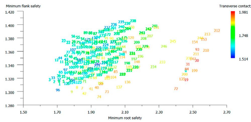
Figure 1—Typical output in commercial software (Ref. 11).

Although this display allows choosing the outputs of interest, focuses the maximum attention on three parameters at a time. Sometimes it is necessary to have more than three variables under control at the same time; with the display as shown in this example, it becomes necessary to change one of the three variables and plot the graph again, losing the previous info. Alternatively, you must save each image separately.

The proposal developed in this paper instead allows for displaying results at the same time. It is possible to choose the number of appropriate variables and get cross-related in between all parameters simultaneously. It is possible to identify possible design trends with project objectives. 

The results obtained are not understood as a process of direct optimization, but as a tool to help the designer identify the solution that best meets the design needs.

To better clarify the reading, the results are reported with gradually increased variables. 

In Figure 2, the correlations between S_H and S_F are reported, adopting the module as a parametric. The use of the fictitious variable of the case study “case” allows having under control the number of the simulation to which reference is made.

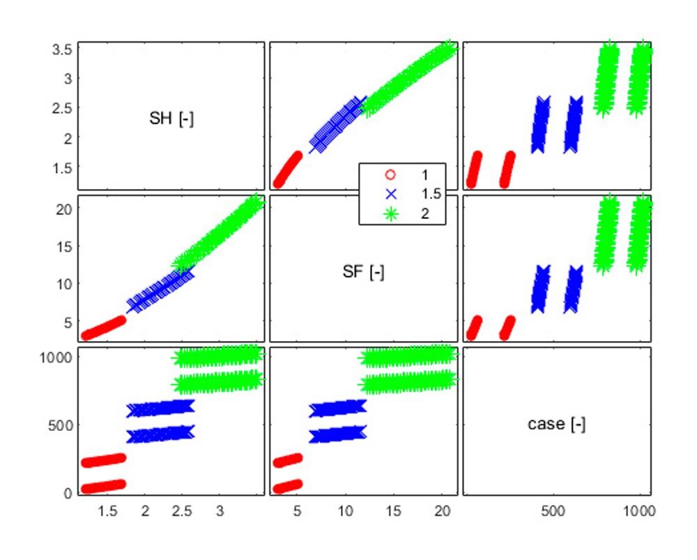
Figure 2—Matrix plot parametrized by module.

It is then possible to increase variables in output, as well as the output ranges to consider.

Figure 3 shows 5 output results for each solution—not taking into account the fictitious variable “case”—and higher number of module parametrized (1.0:0.5:3.5) than Figure 2 (1.0:0.5:2.0) with only 2 output results, S_H and S_F. The results in the figure below are about transmission ratio, external diameter of the sun and type of dynamic response expected in the system.

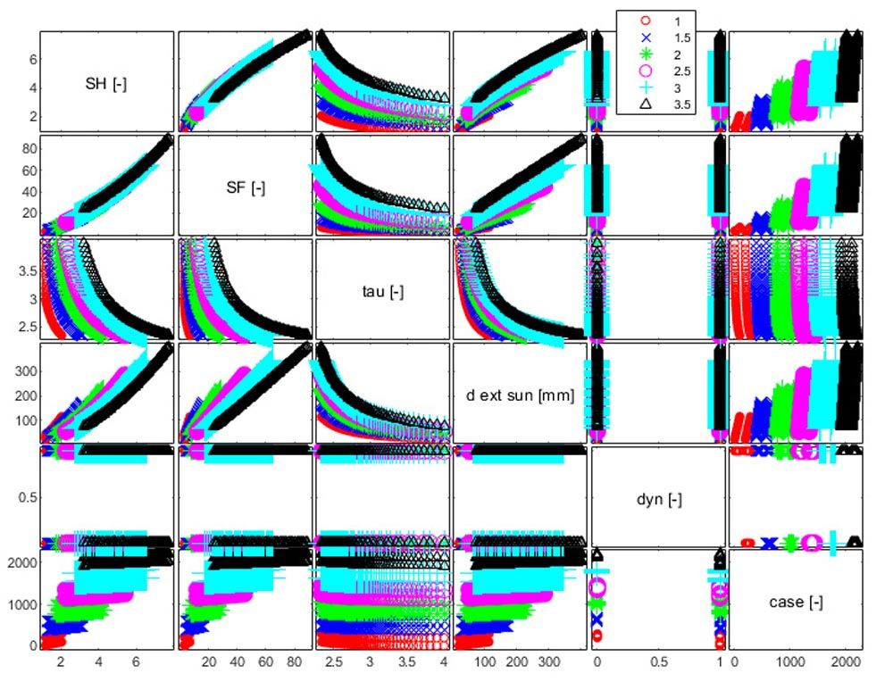
Figure 3—Matrix plot with six parameters.

It is evident how the user can manipulate it: the visualization here proposed allows finding any correlation trend between variables.

At the same time, it is possible to narrow the ranges as happened in Figure 4, restricting the transmission ratios to be displayed by x

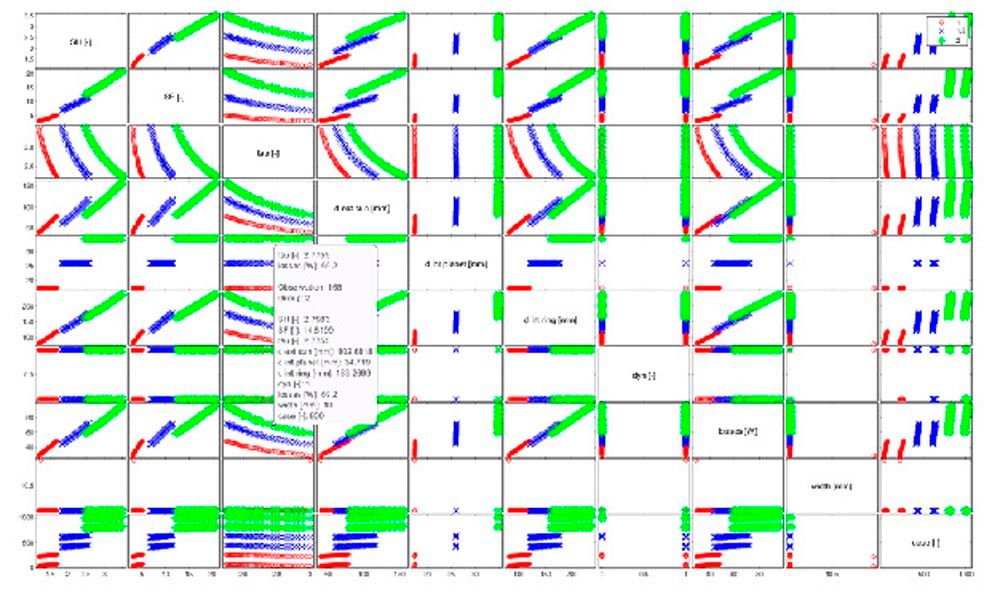
Figure 4—Matrix plot parametrized by module with constrained ranges.

With the procedure indicated, it is possible to store a large number of technical solutions, with an equal level of design accuracy from which to choose the most suitable for this application.

Thanks to this visualization it is easy to evaluate the losses synthetically and identify if there is some parameter driving the loss minimization logic, all while having under control all the design data of every single epicyclic gear train.

To understand the details that can be reached, the inner diameter of the planet and ring have been stored. They may be design limitations in the design phase when choosing such numerical values, to be written to the problems of:

• system dimensions, in the case of the ring diameter;
• support geometry of the planet carrier, in the case of the planet diameter.

In these, are directly available, the analysis of dynamic setting to define that the system is dynamically driven by a kind of forcing instead of another, symmetric or sequential mesh sequence. It is so easy to change the boundary conditions to jump out from the matrix plot, to visualize better the results based on the target. In Figures 3 and 4 the same results shown before are divided by the kinematic forces, in the case 1 instead of 0 for sequential and symmetric solutions respectively.

Moreover, the designer once again chooses the number of constraints. For example, a specific range of transmission ratio can be simply isolated simultaneously also building the type of dynamic response (1 instead of 0), and the root diameter of the ring teeth (

It is possible to parametrize the results based on what the designer wants to see.

The intention is to show how results can be easily shown, focusing on the designer’s interest.

Such charts are to be understood as project maps to help the designer allow the wisest choice of the transmission system to have under control the greatest number of variables.

Future Work

There are therefore many developments that it would be possible to think about. 

Firstly, the automation of the entire process analyzed in this paper could allow the development of a user-friendly black-box package, easy to use for the designer.

Secondly the parametrization of system stiffness, on a geometric basis, allows for calculating the dynamic response of the system; it is in this way to identify which of the forcing dynamics of the system satisfy the designer’s choice (Ref. 5).

The same calculation has already been implemented for the calculations of external gears: joining the two works would allow to extend the analyses also for complex transmission systems. Complex systems could also be considered for a multistage epicyclic gear system.

Conclusion

This paper shows a methodology to extensively evaluate different designs of epicyclic gear systems. 

As outlined, no choice is required on the part of the designer who is free to probe all design variables.

The study was divided into different steps well defined:

1. Selection of variables to be included in the study and the automatic generation of all mathematically possible combinations;
2. Automatic design of each epicyclic system according to geometric constraints and minimum security requirements guaranteed;
3. Results in visualizations according to filtering logic and results sampling.

Acknowledgments

The authors would like to thank KISSsoft and Gleason Corporation for the software used to develop the script described in this paper, Ing. Ivan Saltini for his constant support, and the University of Bologna for the access to bibliographic references.

References

1. Turci, M. and Solimine, V. “Closed Loop for Gears: Some Case Studies.” Paper No. 22FTM11, AGMA Fall Technical Meeting, 2022.
2. Matlab, Software User Manual.
3. Pinnekamp, B. and Hider, M. and Beinstingel, A. “Specific Dynamic Behavior of Planetary Gears.” Paper No. 19FTM26, AGMA Fall Technical Meeting, 2019. 
4. Kahraman, A. “Gear Dynamics and Gear Noise Short Course,” March 21-24 2022. The Ohio State University.
5. ANSI/AGMA 6123-C16, Design Manual for Enclosed Epicyclic Gear Drives.
6. ISO 53:1998(E), Cylindrical gears for general and heavy engineering—Standard basic rack tooth profile.
7. Kissling, U. “Use of duty cycles or measured torque-time data with AGMA ratings.” Paper No. 21FTM07, AGMA Fall Technical Meeting, 2021.
8. Turci, M. “Design and Optimization of a Hybrid Vehicle Transmission.” Paper No. 18FTM06, AGMA Fall Technical Meeting, 2018.
9. ISO 6336-1:2019, Calculation of load capacity of spur and helical gears — Part 1: Basic principles, introduction, and general influence factors.
10. Weber C., Banaschek K.; FVA-Bericht 129 und 134, Elastische Formänderung der Zähne und der anschliessenden Teile der Radkörper von Zahnradgetrieben, FVA 1955.
11. KISSsoft, Software User Manual, 2023.
12. Niemann, G.,Winter, H. Maschinenelemente, Band 2, Berlin: Springer 1983.