All bevel gears are designed using a reference right cone called
the “pitch cone.” The pitch cone is used as a basis for describing
all other geometric entities of the bevel gear. Since describing
the motions of the generating process in three dimensions
would be hard to visualize or comprehend, the general practice
is to un-wrap the surface of the pitch cone into a tangent
plane — or “pitch plane.”
The point at the top of the pitch cone is called the “pitch
apex.” The pitch apex is significant because the axes of both gear
and pinion intersect at this point. Figure 2 displays the pitch
cone, the pitch plane unwrapped, and also describes the global
Cartesian coordinate system, CG. Figure 2 also shows the pitch
cone sectioned through the YZ plane. This describes the definition
of the pitch angle, Γ, and the face width, F — of a part. The
global coordinate system follows the right-hand rule and its origin
is located at the pitch apex of the member being modeled.
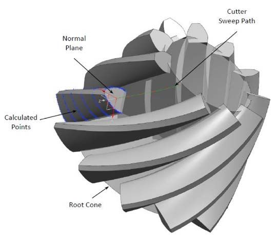
Figure 1 Visual depiction of calculation method.
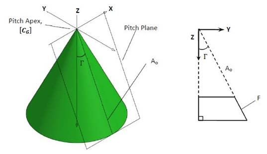
Figure 2 Pitch cone.
Basic Generation
The majority of all generated spiral bevel gears are manufactured
in one of two processes, i.e. — face milling or face hobbing;
both manufacturing methods have advantages and disadvantages.
For the purposes of this method, a brief understanding
of the generating method utilized during these processes is
necessary to realize the 3D model.
Face milling. The face milling manufacturing method
employs a circular, cup-shaped cutting tool moving in a timed
relationship with the workpiece to roll through the gear blank
and generate an individual slot. The cutter is then withdrawn, the work is indexed to the location of the next slot, and the process
repeated. See Figure 3.
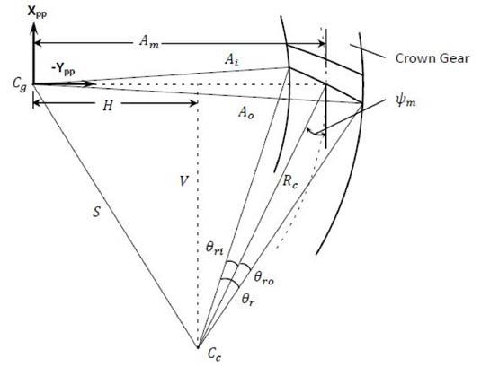
Figure 3 Generating triangle in pitch plane for face milling.
Figure 3 displays three instances of the cutter as it passes
through the workpiece; these points are at the toe, mean, and
heel of the crown gear. The path of the cutter sweeps a circular
arc in the lengthwise direction, with the same radius as the
radius of the cutter, Rc. The axis of the crown gear, Cg, is known
as the machine center. The local coordinate system for the pitch
plane is located at the machine center. Xpp correlates to X and
Ypp lies along the line describing Ao in Figure 2.
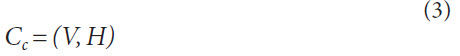
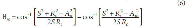
The cutter axis, Cc. This location can be found by:
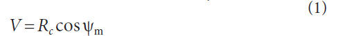
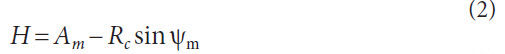
The sign of the vertical term, V, may either be positive or negative,
depending on the hand of spiral to be modeled. Figure 3
shows a right-hand member (use negative value for V when calculating
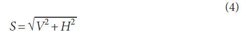
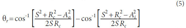
left-hand members). The cutter sweep angle, θr, is necessary
to determine how much rotation is used during the cutting
process. When calculating points to model the gear tooth,
these will be the endpoints of the working portion of the cutter
path.
Discrete points can be calculated along the cutter sweep on
the pitch plane. Using the general parametric formulas for a circle,
the solution for a point, p, along the cutter path is:
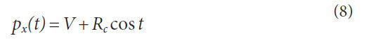
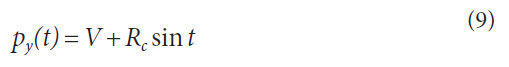
Where t is a parameter that has the following ranges:
For left-hand members,
For right-hand members,
This cutter path can be broken into as many discrete sections
as desired.
Face hobbing. The face hobbing manufacturing method is
a continuously indexing process. The cutting tool has groups
of staggered blades; the workpiece moves in a timed relationship
with the cutter so that a group of blades in the cutter passes
through a slot of the workpiece. The face hobbing method generates
an extended epicycloidal shape in the lengthwise direction.
See Figure 4. for a detailed layout of the face hobbing generating
triangle.
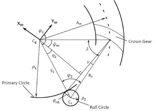
Figure 4 Generating triangle in pitch plane for face hobbing.
Since the lengthwise shape of a face hobbed part creates an
extended, epicycloidal shape, a little trigonometry is necessary
to calculate the discrete points along the path created by the cutter.
The crown gear tooth count,
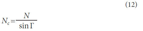
The lead angle of the cutter,

The first auxiliary angle,
The center distance from crown gear center to cutter (Radial),
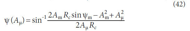
The second auxiliary angle,
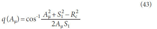
The second roll angle,

The auxiliary roll angle,
The radius of the roll circle,
The radius of the primary circle,
The first roll angle (assuming rolling without sliding),
Now that the dimensions of the cutting cycle’s epicycloid,
the cutter path, can be calculated, it would be very difficult to
determine the angle of sweep that the cutter makes during the
generating process because the cutter axis does not remain stationary
during the cutting cycle. The face width of the bevel gear
being modeled will be subdivided into discrete portions; the roll
angles need to be recalculated for each discrete location individually.
The second roll angle as a function of cone distance,
Where,
The first roll angle as a function of cone distance,
The local Cartesian coordinates describing a point, p, along
the cutter sweep path can be calculated.

Wrapping the Pitch Plane
The pitch plane is a tangent plane to the lateral surface of a right
cone. This cone, as described earlier, is the “pitch cone.” The
diagrams take into account the set-up of the machine, the cutter
size, and the motion of the cutter. Rotation of the workpiece
also needs to be accounted for; this is accomplished by wrapping
the pitch plane around the pitch cone. This transforms the
local coordinates calculated for the cutter sweep path into global
coordinates. These points in the global coordinates will define
the center of a tooth slot. The following formulas will transform
a point, p, from the local XppYpp plane to the global Cartesian
coordinate system, CG.
The first step is to determine the location of the point in the
global Z axis direction,
Calculate the rotation angle that the point will wrap around
the cone,
Calculate the radius of the cone at location, Zp,
Convert the cylindrical coordinates for the wrap point into
global Cartesian coordinates.
Therefore, all the local cutter positions can be wrapped and
transformed into the global Cartesian coordinate system.
Calculating Local Cutter Coordinate System
Since AGMA 929 effectively calculates the normal circular tooth
thicknesses at a specific spot along the cutter path, the next step
is to determine the correct orientation of the normal plane. A
complete coordinate system will be oriented to have the xnyn
plane normal to the cutter path, with the origin at each global
coordinate of the cutter path calculated previously; this coordinate
system will be called Cn.
Tangent axis, zn. The tangent axis is defined by a vector that is
tangent to the cutter sweep path at the location of the wrapped
point. There are a couple of options for calculating this tangent
vector. One could calculate the first derivative of the cutter
sweep path formulas for both face milling and face hobbing
so that the slope anywhere along that path can be predicted.
Once that is accomplished a vector can be constructed in three
dimensions to describe this tangent axis.
Since many assumptions are made throughout this method,
the simplest method for calculating an approximate tangent
vector is using finite difference; the finite difference method is
described in the following equation:
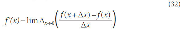
It is difficult to determine the correct size of Δx that will
approximate the tangent close enough for this method. Since
the cutter sweep path is smooth and continuous for all locations along the arc, it is possible to quantify the error of our approximation
using a Taylor expansion. This is beyond the scope of
this document, but is mentioned here for further exploration.
The practical approach to applying the finite difference method
is to calculate a neighboring wrapped point along the cutter
sweep path for each wrapped calculation point. A vector can
then be defined by passing through both sweep path points. As
the points become closer and closer the vector connecting the
two points approaches a tangent line.
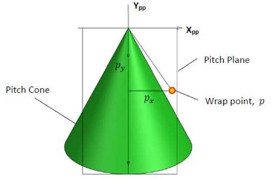
Figure 4 Generating triangle in pitch plane for face hobbing.
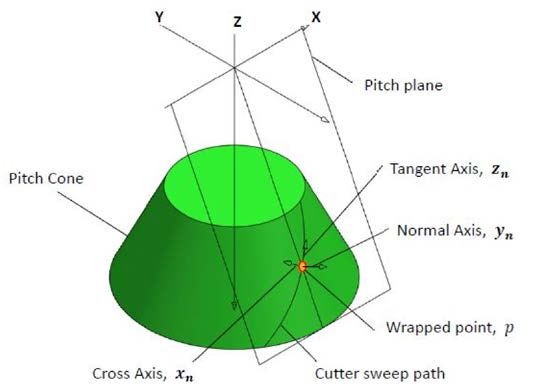
Figure 4 Generating triangle in pitch plane for face hobbing.
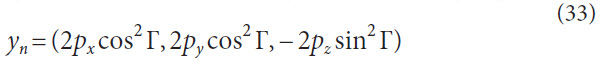
Normal axis — yn. The normal vector is defined as a vector
radiating perpendicularly from the surface of the right cone at
the wrapped point location (Fig. 6). The normal vector at wrap
point p = (px, py, pz) can be calculated by the following equation:
A brief derivation will follow to explain the calculation of the
normal axis. The general function of a right cone,
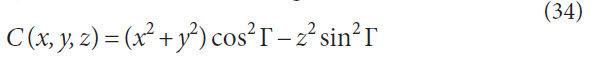
A gradient, u, is always normal to a function when,

Where,
Let,
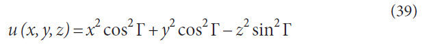
Therefore,
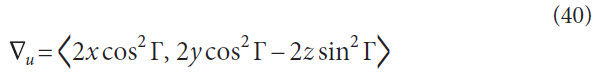
The cross vector will complete the definition of the local
Cartesian coordinate system. This vector is calculated by taking
the cross product of the tangent vector and the normal vector.
After calculating all the vector directions for the local coordinate
system, all three of the vectors should be normalized.
Normal Circular Tooth Thickness Calculations
Generalizing AGMA 929-A06. As previously discussed AGMA
929-A06 utilizes the technique of converting the spiral bevel
gear tooth to a virtual spur gear tooth to calculate the top lands
at the toe, mean, and heel; the equations presented in AGMA
929-A06 are unique for each of these points of interest. General
equations can be derived from AGMA 929-A06 so that the
tooth thickness can be calculated anywhere along the profile
and lengthwise direction. The generalized formulas for the conversion
to a virtual spur gear are presented here (Fig. 7).
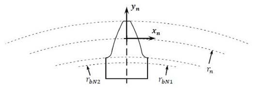
Figure 7 Definition of the geometry of the virtual spur gear in the
normal plane.
Also,
a handful of helpful formulas for calculating some spiral gear
tooth geometry with respect to cone distance,
Aμ, are developed.
The cone distance range variable must correlate to the cone distances
first chosen in the cutter path sections.
The notation in this section utilizes the terminology as if the
member being modeled is the gear. Unless specifically specified
the gear terminology should be replaced with pinion terminology
in the formulas if the pinion is the part being modeled.
Spiral angle for face milling with respect to cone distance,
Generating angle for face hobbing with respect to cone distance,
Spiral angle for face hobbing with respect to cone distance

Slot width with respect to cone distance for the gear member,
Slot width with respect to cone distance for the pinion member,
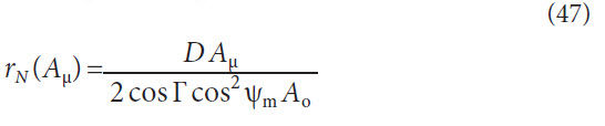
Normal pitch radius with respect to cone distance (substitute
proper pitch diameter and pitch angle for member to model),
Normal base radius with respect to cone distance, concave,
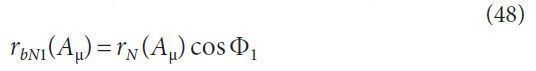
Normal base radius with respect to cone distance, convex,
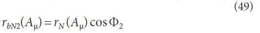
Figure 7 displays the base radii graphically. The value of rrbN1
and rbN2 are shown as the same value because the pressure angle
of the concave and convex flanks are the same. This is typical
but not mandatory for bevel gears without a hypoid offset.
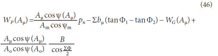
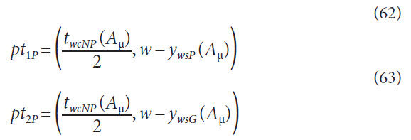
Normal pinion circular tooth thickness at pitch line with
respect to cone distance,
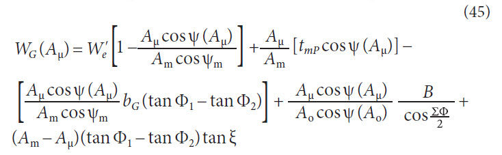
Normal gear circular tooth thickness at pitch line with respect
to cone distance,
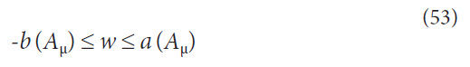
Normal working radius with respect to cone distance,

Where
w is a range variable for calculating the working radius. The
valid range for w is,
Pressure angle at working radius with respect to cone distance,
concave,
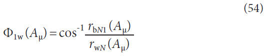
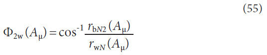
Pressure angle at working radius with respect to cone distance,
convex,
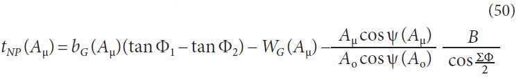
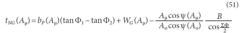
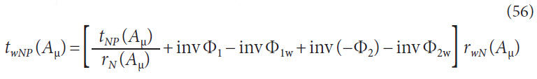
Normal circular tooth thickness for pinion at working radius
with respect to cone distance,
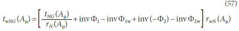
Normal circular tooth thickness for gear at working radius
with respect to cone distance,
Certain designs have the dedendum plunge below the virtual
gear’s base radius; when this occurs, the normal circular tooth
thickness will become a complex number. Only the real portion
of this value should be used when recording the answers.
Converting thicknesses to coordinates. The tooth thickness
calculations shown earlier in Generalizing AGMA 929-A06 is a
circular tooth thickness positioned at a specified working radius.
The local coordinate system has the origin located where the
pitch radius crosses the center of the tooth thickness (Fig. 7). For
each working radius used the calculated circular tooth thicknesses
need to be converted to chordal thicknesses before they
can be recorded as Cartesian coordinates.
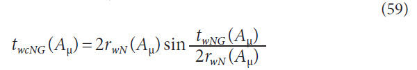
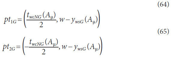
Normal chordal tooth thickness for pinion at working radius
with respect to cone distance,
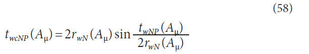
Normal chordal tooth thickness for gear at working radius
with respect to cone distance,
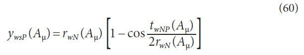
Now that the circular thickness has been converted to a
chordal thickness, a small correction is needed to the location of
the thickness in the profile direction (along yn). Figure 8 depicts
this correction and provides a visual explanation why this correction
is required. The working radius is equal to the pitch
radius in the figure, and its relative radius has been decreased to
exaggerate the size of the correction in the figure.
Pinion shift factor at working distance with respect to cone
distance,
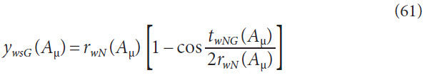
Gear shift factor at working distance with respect to cone distance,
Local Cartesian coordinates for the pinion with respect to
cone distance,
Local Cartesian coordinates for the gear with respect to cone
distance,
Transform the Local Normal Tooth Thicknesses to
Global
To this point all the tooth thickness points are defined relative
to a local coordinate system. The global location for each one
of these local coordinate systems are known, but to complete
the model, all points describing the tooth flanks must be known
relative to the global coordinate system. This is accomplished
using a coordinate transformation matrix, CT:
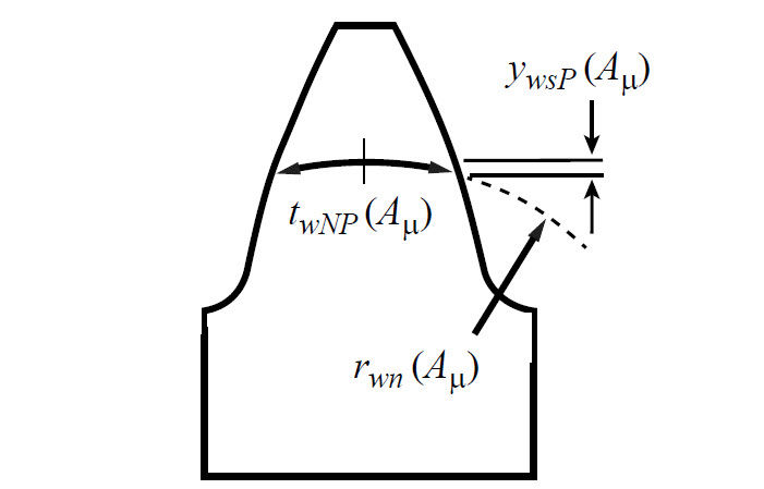
Figure 8 Shift factor when converting
circular to chordal thicknesses
(pinion shown).
Where,
CG is a 3×3 identity matrix that describes the global coordinate
system. See Coordinate System Definition for a more
detailed explanation. Once a vector, Vp, relative to the local coordinate system, Cn, is constructed that passes through a calculated
tooth flank point, the transformation can be calculated:
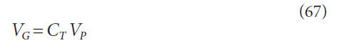
Where,
VG is a vector that passes through the exact same flank point,
but is described relative to the global coordinate system.
Results
Now that the method is complete, the next logical step is to
determine just how accurate this model is when compared to
the theoretical geometry of a spiral bevel gear. This method is
strictly approximate; many caveats have been discussed in the
previous sections. To accomplish a comparison between this
method and a theoretical part there must be a reliable standard
by which to compare it. Comparing the calculated points from
this method with a physical, cut part would introduce potential
variations from the manufacturing process. For this reason
alone it was decided to compare the calculated points to a different,
yet trusted, mathematical model. Gleason Works has developed
a commercial software package — T900 — that generates
an accurate point cloud describing the geometry of the tooth
flank and fillet condition of bevel gears and pinions. While the
purpose of this software is far greater than just the generation
of a point cloud, the other functionality is beyond the scope of
this document. The point cloud produced from T900 can be
imported into a CAD package to assist in the generation of the
exact geometry produced by the machine settings
for a particular design. The point cloud represents
the standard as to which this method is compared.
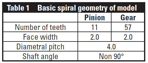
The member chosen for this analysis is a left-hand
spiral bevel gear generated by face mill completing.
Some of the basic geometry has been provided in
Table 1, but the exact details of the geometry are relatively
unimportant. An angular set was chosen as this
method has no shaft angle restrictions.
The output from T900 is a point cloud that
describes the flanks of a spiral bevel or hypoid gear
set. A gear tooth is divided into a 13- (profile) by-10
(length) grid for each flank; therefore 260 unique
points describe each tooth. For this analysis these
discrete points were bridged together using Siemens
NX 8.5 CAD software. The point cloud was connected
in the profile and lengthwise direction with
curves generated by a cubic, polynomial regression.
Once the lattice of curves is generated the curves
are used as ribs to create a bi-cubic surface. Figure
9 shows the tooth surface generated from the T900
point cloud in gray.
The face width of the part is broken into 10 segments
for the calculation; addendum and dedendum
are also broken into 10 segments. The part being modeled has a
short addendum and long dedendum. Figure 10 shows the calculated
points and solid model sectioned through the normal
plane (Fig. 9) of a tooth.
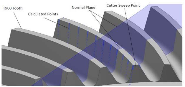
Figure 9 Calculated points overlaid on a tooth modeled using Gleason
T900.
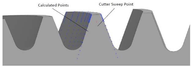
Figure 10 Calculated points in the normal plane.
The calculated points go beyond the
root line of the model because the calculated points were generated
to the base circle radius of the virtual spur gear. When
doing the comparison the last four points of each profile will be
omitted, as they fall below the root fillet tangency point.
A linear measurement normal to the T900 surface to each calculated
point is used to measure the deviation between the calculated
points and the surface. The normal tooth thicknesses
at the toe and heel will be omitted in the comparison, as these
points are beyond the bounds of the T900 surface. The absolute
values of the measured deviations for each flank are given
(Tables 2 and 3).
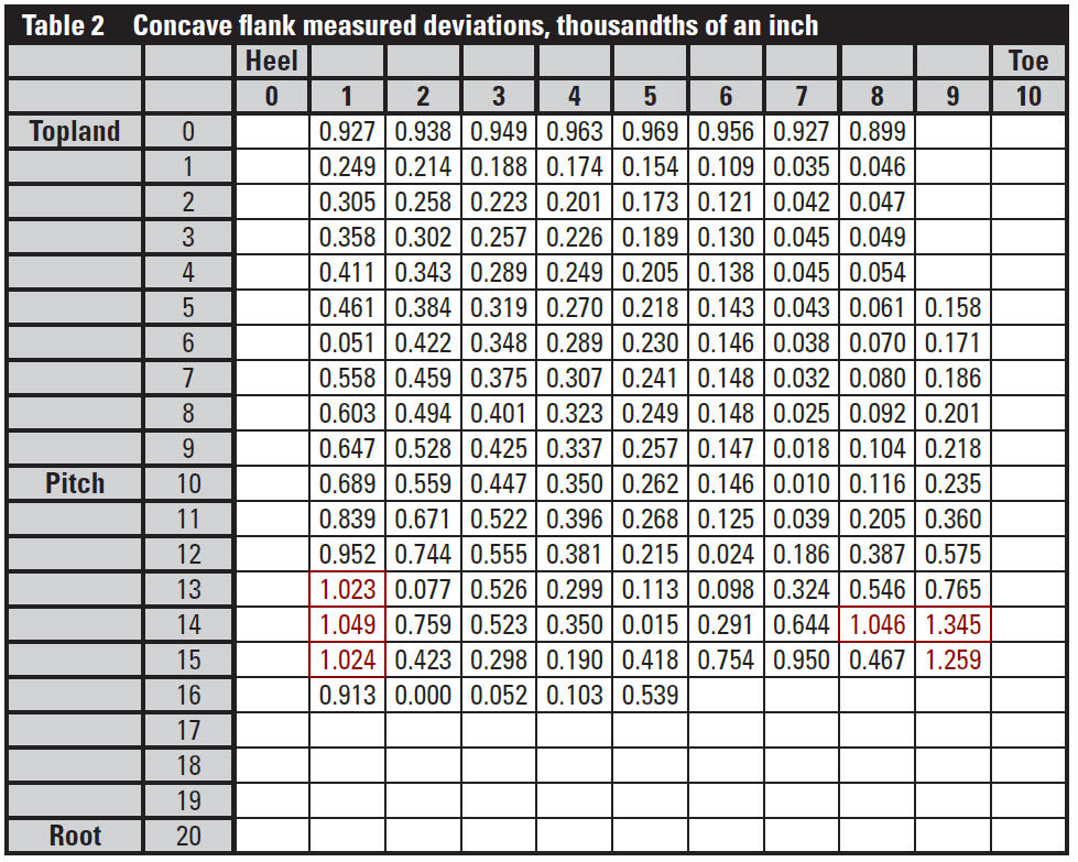
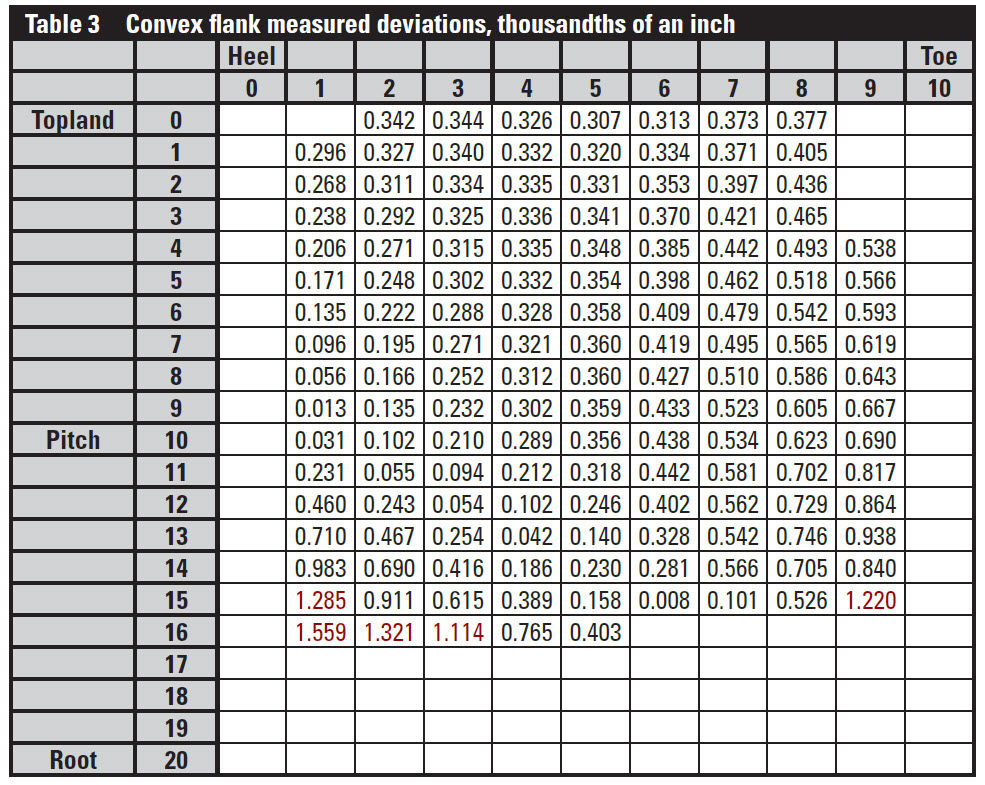
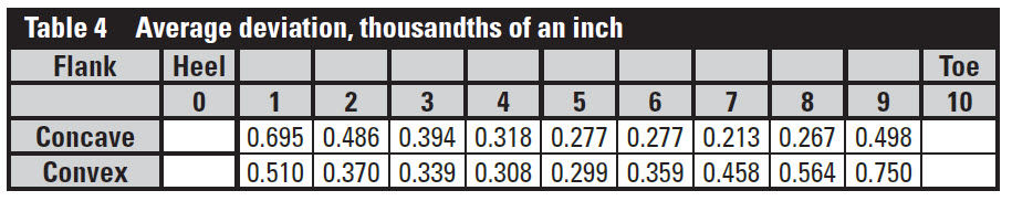
The red values are measured deviations that exceed one onethousandth
of an inch. Overall, the results depict a model that
very closely approximates the flanks predicted by the Gleason
Works T900 software. The average deviation for each normal
cross-section in the lengthwise direction is displayed in Table 4.
Conclusion
The purpose of this presentation is to describe a procedure for
calculating a very close approximation of the geometry of a spiral
bevel gear tooth.
This method is built upon the techniques and formulas
described in AGMA 929-A06.
The second portion of the document compared the results of
this method with the results from a proven Gleason software
package.
The results are extremely close.
Many models have been generated since this original case
study, and the subsequent models correlate well with the geometry
predicted by Gleason software.
The model described throughout this document
should not be used for advanced analysis
(i.e., finite element or the like), as the models
created from this method do not have any modifications
to the tooth flanks to adjust or optimize
the tooth contact pattern.
At present AGMA’s Bevel Gear Committee
is working on revising the formulas in AGMA
929-A06 to adopt the generalized formulas
described here. The technique of utilizing generalized
formulas will expand the capabilities of
AGMA 929.

After graduating from
Northern Illinois University
in 2010 with a bachelors’ in
mechanical engineering,
Brendan Bijonowski
has pursued a career in
design. In 2011 he joined the
engineering ranks of Arrow
Gear Company, located in Downers Grove,
IL as a design engineer. His passion for the
geometry of gearing and attention to detail can
clearly be seen in all of his work. Bijonowski is
a member of the AGMA Bevel Gear Committee,
where he works on defining geometry and
improving rating methods. He is also a
member of the AGMA Computer Programming
Committee, where he applies his experience
and knowledge as a gear engineer to an evergrowing
collection of technical software.
References:
- Baxter, Jr., M.L. Spiral Bevel Gear Theory, Unpublished.
1963.
- AGMA 929-A06. Calculation of Bevel Gear Top Land and
Guidance on Cutter Edge Radius.
- Colbourne, J.R. The Geometry of Involute Gears,
Springer-Verlag, New York, 1987.
- ANSI/AGMA 2005-D03. Design Manual for Bevel Gears.
- Grant, G.B. A Treatise on Gear Wheels, 21st Edition.
Philadelphia Gear Works Inc., Philadelphia, 1980.
- Khiralla, T.W. On the Geometry of External Involute Spur
Gears, C/I Leaming, North Hollywood, California, 1976.
- Krenzer, T. The Bevel Gear, 2007.
- Litvin, F.L. Theory of Gearing, NASA Reference
Publication; 1212 (AVSCOM Technical Report; 88-C-
035), 1989.
- NX 8.5 Help Documentation. Siemens Product Lifecycle
Management Software Inc., 2012.
1- Shtipelman, B.A. Design and Manufacture of Hypoid
Gears, John Wiley and Sons, Inc. 1978.
-
T900 User’s Manual. Gleason Works.