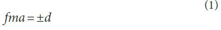
Also, we may express the resulting error, fma, as a probability
density function as follows:
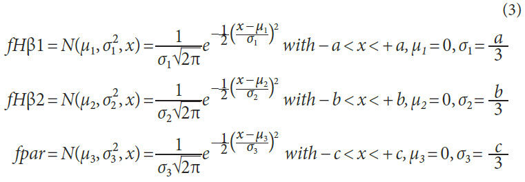
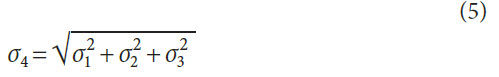
Because fHβ1, fHβ2 and fpar are independent of each other,
we find the standard deviation σ4 as follows:
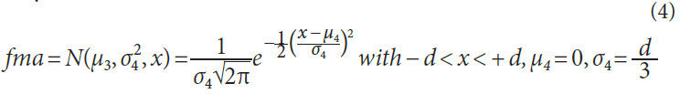
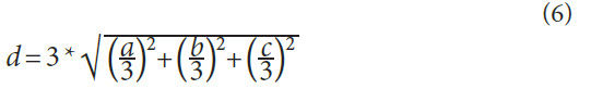
Again assuming that 3-Sigma rule applies for fma
(i.e. — d = 3*σ4) we find:
And
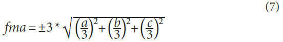
Which means that after assembly, 99.73% of all gearboxes
have a total misalignment of the flanks with respect to each other of fma = ±d — where d is calculated using the
above formula.
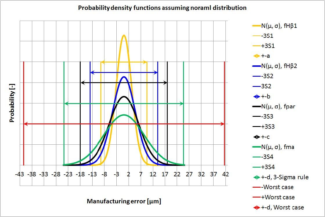
Figure 1 Normal distribution of manufacturing errors, resulting error, and worst-case scenario.
The above relationships are shown in Figure 1.
The probability density functions (assumed
to be normal distributions) of the three basic
errors — fHβ1, fHβ2 and fpar — are shown in
orange, blue and black. Also shown are the tolerances
±a, ±b, ±d corresponding to ±3*σ1, ±3*σ, ±3*σ3
(where σ is the standard deviation).
Combining these three random errors, we find the probability
density function (again assumed to be a normal distribution)
of the resulting error fma in green. Also shown is the tolerance
±d corresponding to ±3*σ4.
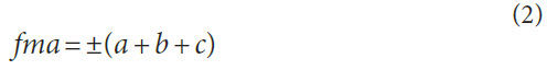
For comparison, the worst-case scenario where d = a + b + c is
shown in red.
We can clearly see that if we use the worst-case scenario, the
value for d is much higher than the value for d, were we to use a
statistical approach.
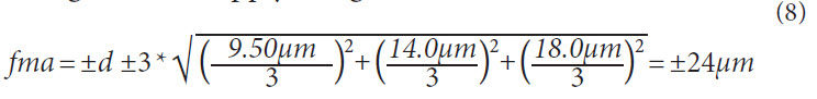
Applying the above formulas we find that the resulting tolerance
range ±d if we apply 3-Sigma Rule as:
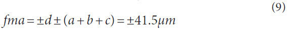
And if we apply a worst-case scenario, we find:
Considering the above statement that the worst-case
approach is considered as overly conservative, then, for the
above gear pair, we would consider a random manufacturing
error in the mesh of fma = ±d = ±24.7μm, when calculating KHβ
along ISO6336-1, Annex E.
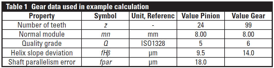
KHβ calculation using statistical or worst-case scenario for
fma. Let us consider again the above gear example. We apply
helix angle modifications on the pinion such that we compensate
the shaft bending, shaft torsion and bearing deformation.
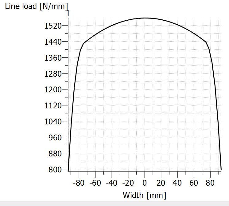
Figure 2 Line load distribution in the mesh for the example — not
considering any random manufacturing errors; KHβ = 1.08.
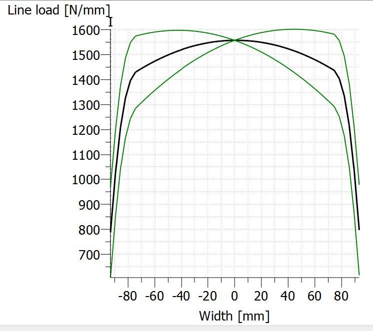
Figure 3 Line load distribution considering random manufacturing
errors fma = ±24.7μm (green lines); KHβ = 1.11; highest line load
occurs well within the crowned area of the face width; design
considered suitable.
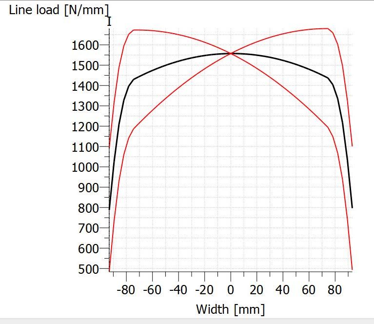
Figure 4 Line load distribution considering random manufacturing errors
fma = ±41.5μm (red lines); KHβ = 1.16; highest load occurs in
the transition area between crowning and end relief; design
considered as not suitable.
The result is a symmetrical line load distribution, calculated
along ISO6336-1, Annex E. If we ignore the random manufacturing
error (assuming fHβ1 = fHβ2 = fpar = 0.0μm), the load
distribution is then symmetrical and highest value lies in the
middle of the gear face width due to an applied crowning of
Cβ = 20μm. Let us also apply a curved end relief over 10% of
the gear face width per side; the amount is CβI = CβII = 45.0μm
(notations as per ISO21771 apply).
The resulting line load distribution is shown below, the
resulting face load distribution factor is KHβ = 1.08.
If we now consider the random manufacturing error
fma = ±24.7μm (from the 3 Sigma-Rule), we find three line
load distributions (one without manufacturing error, one using
fma = +24.7μm, and fma = −24.7μm), as shown below. The face
load distribution factor has now increased to KHβ = 1.11. And
yet, the highest line load remains within the crowned part of
the face width; thus the design would be deemed quite acceptable.
But if we consider the worst-case manufacturing
error — fma = ±41.5μm — we find the below line load distributions.
The face load factor is now KHβ = 1.16 and we find that
the highest line load is just where the end relief is about to start,
thus rendering the design unacceptable in this case.
Conclusion
 Hans-Peter Dinner
 studied mechanical
engineering at the Swiss Federal Institute
of Technology (ETH), where during his
studies he spent time with Mercedes
Benz working on FEM of car bodies; with
Buhler in South Africa for training; and
with the National University of Singapore
for writing his thesis on FEM analysis
of medical devices. He began as an
FEM engineer, working with the leading
consultant in Switzerland on welded
structures, pressure vessels and satellite structures. Dinner later joined a
leading roller coaster design company, being responsible for all strength
verifications. He then moved on to KISSsoft AG, supporting customers in
the use of their gear software, working on gear optimization projects, and
ultimately transitioning to sales of KISSsoft products, with a focus on the
Asian market. In 2008 he started his own consultancy firm, EES KISSsoft
GmbH, sharing his time between KISSsoft support and sales in Asia and
project work. Key projects included design and testing of SCD3MW and
SCD6MW wind gearboxes, and large-bearing calculations for cranes and
wind turbines as well as gear optimizations for sugar mills, vertical roller
mills and tractors. Dinner’s main interests are planetary gearboxes, tooth
contact analysis and testing.
An easy-to-use approach has been presented showing how random
gear helix slope deviations and shaft parallelism errors
due to housing errors can be considered in the calculation of KHβ. It is shown that adding up all random errors in a worstcase
scenario is overly conservative. Applying the 3-Sigma
Rule, errors may be combined in a different way such that the
resulting error covers 99.73% of all cases. The difference in the
resulting KHβ values when using this worst-case approach (in
the above example, KHβ = 1.16) vs. the more realistic statistical
approach (KHβ = 1.11) is significant when optimizing a design.
The use of the above statistical approach in consideration of
manufacturing errors in the calculation of KHβ along ISO6336-
1, Annex E or AGMA927 is recommended.
A word of caution: experience shows that when designing gear
lead modifications, or when calculating gear load distributions,
much attention should also be paid to the bearing deformation
and variation in bearing operating clearance. These effects are
not elaborated above, but are summarized in the error fpar.